Reimplementing 4DFlowNet
This post analyzes the 4DFlowNet (2020) paper and presents experiments on its upscaling layer, improving the MAE score compared to the original baseline [1].
Introduction
The goal of this paper is to improve the spatial 4D flow MRI resolution. 4D Flow MRI measures the velocity of blood in the body but is subject to noise and low resolution. 4D Flow MRI scans from real patients (real datasets) are expensive, which is why the authors created a synthetic dataset pipeline that generates realistic low-resolution 16x16x16 MRI patches from a high-quality simulation of the aorta using computational fluid dynamics (CFD). These simulated scans were upscaled with an image super-resolution network that was adapted to 4D flow MRI velocity field representations. The 4D FlowNet results showed a relative flow rate errors of 0.6–5.8% and 1.1–3.8% in the phantom data and normal volunteer data, respectively.
Methodology
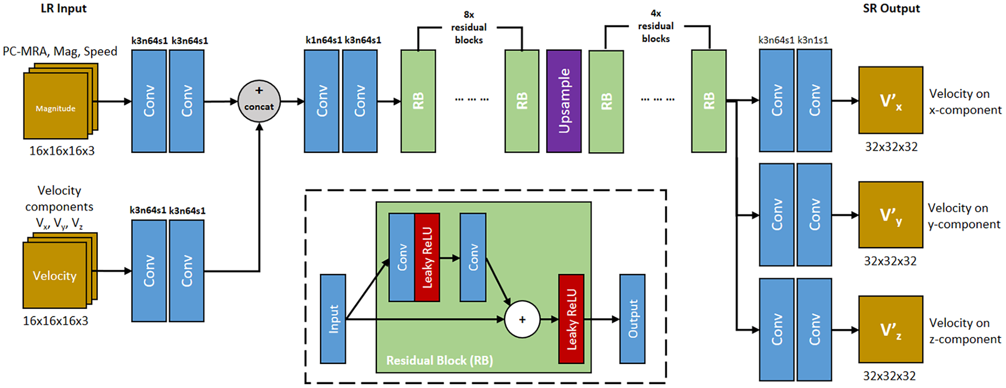
The Network architecture is based on the generator of the super-resolution residual network (ResNet) paper [2]. The input has one path for the raw noisy velocity maps (16^3) and one that accepts calculated context: Magnitude, Velocities and PC-MRA (=Mag*Speed). Both of them pass through two convolutional layers and are then concatenated. Then they are passed through 8 residual blocks (RB). Each RB consists of two conv layers with a nonlinear layer in between and a skip-connection after which another Leaky ReLU is used. After the 8 RB-layers 64 semantically rich feature maps are upsampled using a simple trilinear resize layer, which is what we will revisit in our experiments later. After upscaling the features pass through 4 more RBs and three two-layer convolutional heads, for each xyz component, that reduce the 64 channels back into one channel of size 32^3.
The loss function consists of a simple mean-squared error (MSE) loss, that compares the upsampled velocity components with their ground-truth and with a velocity gradient (VG) term. While the MSE loss indicates the vector magnitude error, byitself it can lead to blurry images because it misses high-frequency spatial velocity shifts and leads to poor performance close to the vessel walls (where velocities slow down). The VG loss counteracts that by rewarding accurate directional derivatives between adjacent velocity vectors.
\[L_{total} = l_{MSE} + 10^{-3} \cdot l_{VG}\]Synthetically generating accurate 4D MRI images is important to transfer good performance learned during training to real patient 4D flow MRIs. Initally they have a real 3D model of the aorta, that is fed into a computational fluid dynamics system, that can model the blood movement. They use a pulse and sample the fine ground truth over time. In order to simulate the noise that a real flow MRI comes with, they add a specific Rayleigh noise, which I explain later in the post.
Fun Fact: They used Blender to create the thoracic aorta 3D models that are the basis for the CFD simulations.
The Metrics that were used in the paper are relative speed error, which compares the predicted speed with the ground truth, net flow rate (mL/s), which is calculated by integrating the velocity vectors passing through a cross-section plane and the divergence field which tracks how well the model preserves the divergence-free nature of an incompressible fluid.
Paper Results
The results showed that the 4D FlowNet outperformed traditional mathematical interpolation methods (Linear, Cubic, Sinc). These were struggling especially during low-velocity phases, while 4D FlowNet was not. Additionally, upsampling a scan of an in vivo aorta from a healthy volunteer cleanly predicted the tissue boundaries and had only small hit in performance.
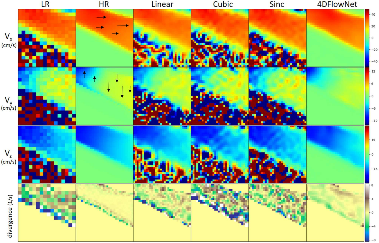
The visual breakdown above showcases how the 4D FlowNet outperforms simple upsampling baselines. While the math-based interpolation methods upsample the noise, the super-resolution generator learned how to effectively subtract the noise, improve the quality, and even implicitly model the fluid’s divergence properties.
Revisiting PixelShuffle for 4D Flow MRI Super-Resolution
While planning how to recreate the paper, I stumbled upon one discussion point on Page 12: the authors actually wanted to use PixelShuffle (sub-pixel convolution) upscaling but rejected it. They reasoned that for sub-pixel convolutions/Pixel Shuffle upscaling on 3D MRI patches, caused (1) poor training convergence and (2) severe checkerboard artifacts.
But before coming to the experiment, I’ll explain how the simplified1 dataset was produced with MRI-specific Rayleigh noise.
The synthetic dataset was created using a 3D mask of a malformed tube and by heuristically generating velocity vectors inside of it. The border tissue of the blood vessel (mask) with a mid-section narrowing (sometimes stronger/weaker) is the base of the MRI patches. After picking the general direction of the blood flow, a main flow close to the center is chosen which has the peak velocity, while blood flow close to the edges becomes slower. Ultimately, I introduced swirl effects that slightly tilt the bloodflow vectors, similar to real fluids.
The k-space is used exactly like in the paper to introduce MRI-specific noise. First, the MRI patches are transformed into a complex MRI signal, using a fast Fourier transform (FFT). Then the outer high-frequency is cropped, which effectively downsamples the patch from 32^3 to 16^3. This complex patch is then corrupted with a randomized signal-to-noise ratio (SNR) of 14-17 dB. This is exactly what produces the MRI-specific Rayleigh-distributed noise, when the patches are transformed back into the spatial domain.
The experiments consisted of comparing the trilinear upsampling layer used in the paper with a PixelShuffle [3] upsampling layer that was mentioned in the Discussion [1]. While the authors had mentioned some drawbacks, I intended to tackle the problems (1,2) by:
- Using modern deep-learning methods that were not used in the paper: AdamW optimizer (they used Adam), cosine annealing LR schedule and gradient clipping.
- Initializing the convolution weights with ICNR (Initialize to Convolution NN Resize) which initializes sub-pixel groups consistently to reduce uneven initial outputs and ensures at least during early training that the model upsamples smoothly [4]. All experiments were conducted on an A100 on Google Colab with a batch of 8 and the final results are in the end of the blog.
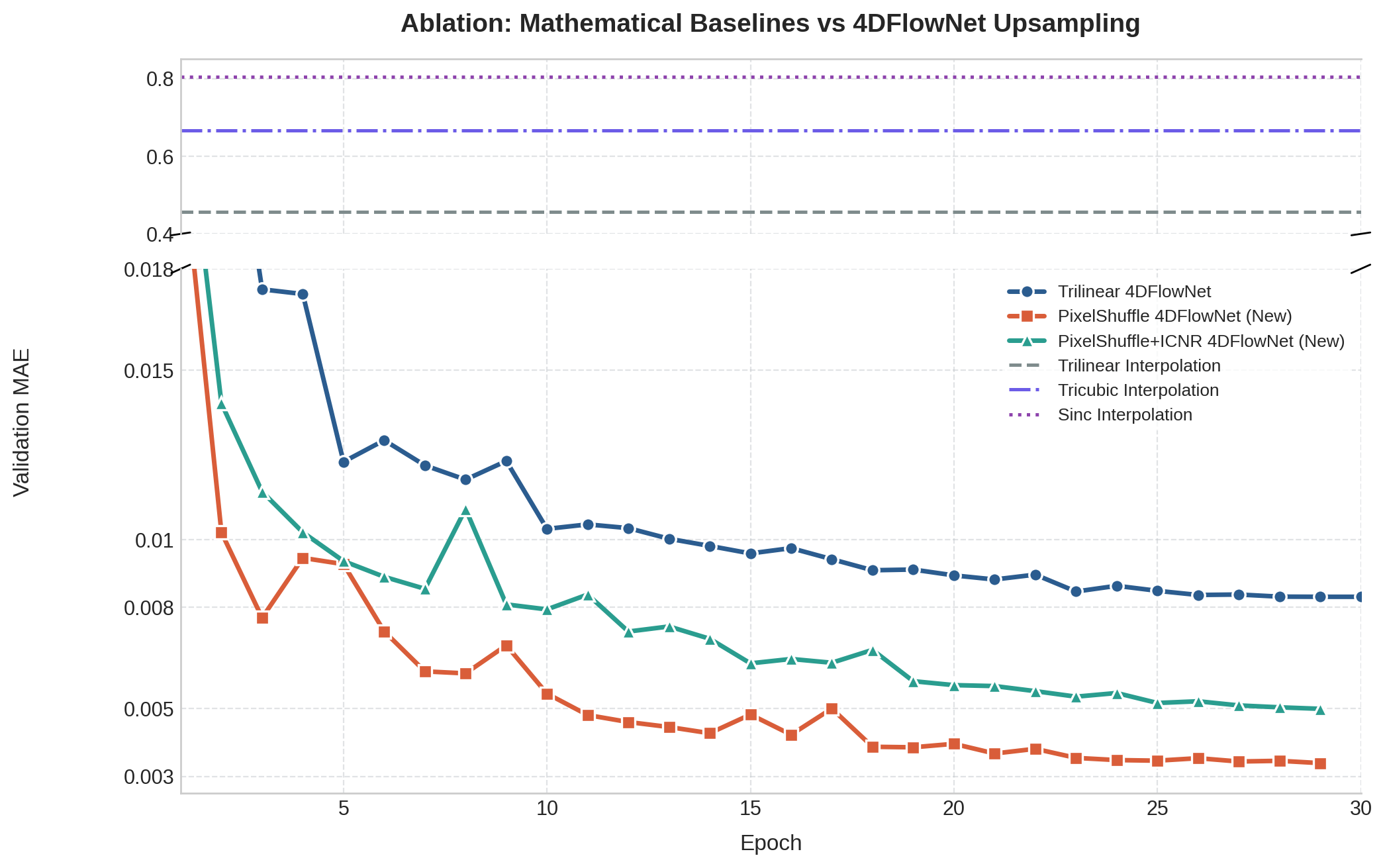
The results confirmed the paper’s concerns and, although MAE, flow velocities and peak flows improved, the divergence score increased by a relative 16-20% and checkerboard artifacts increased 80-120% even with ICNR initialization.
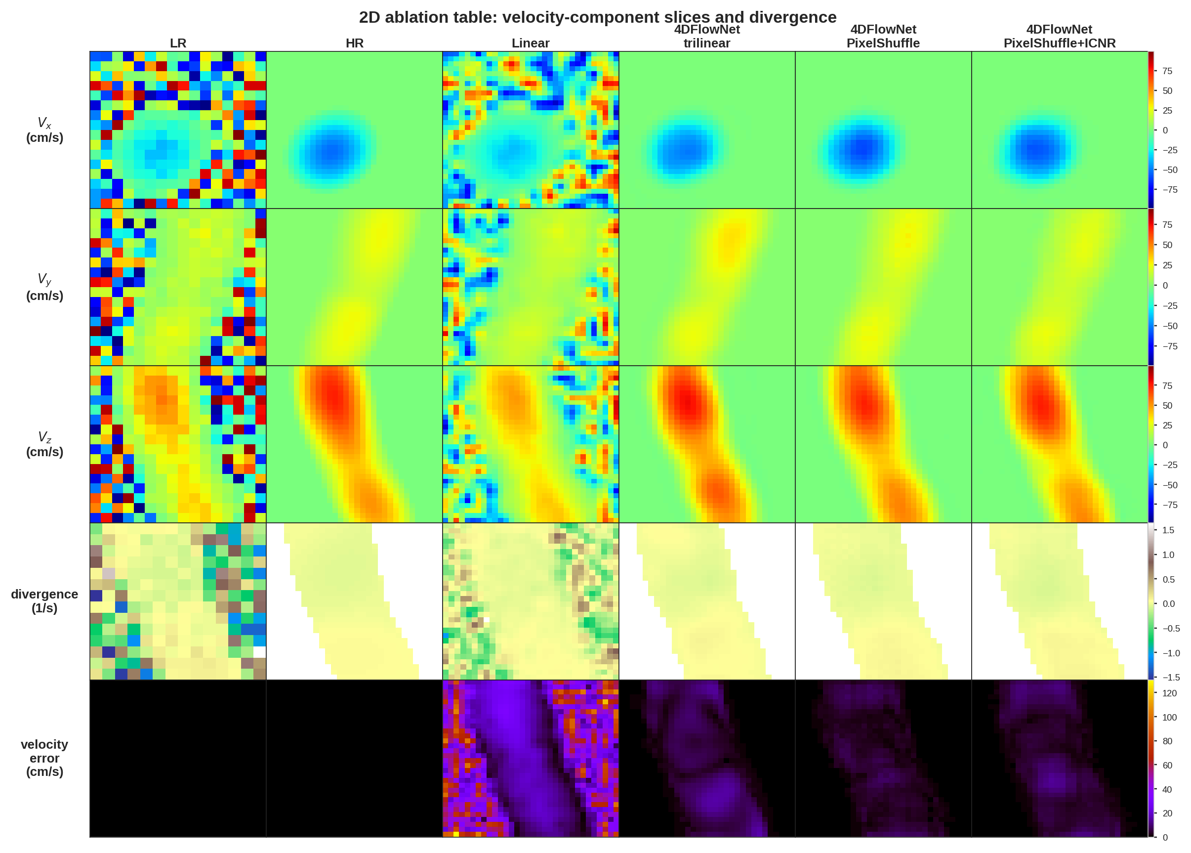
The recreated table above shows all 4D FlowNet implementations beat the Linear method quite clearly, there is a visible difference in the velocity error row between trilinear and PixelShuffle upsampling, where trilinear upsampling performs worse.
Conclusion
I present a summary of 4D FlowNet, which upsamples and denoises 4D Flow MRI patches. The official 4D FlowNet was exclusively trained on synthetic phase and magnitude images generated from CFD simulations and generalizes well on healty volunteer data. Additionally, I conducted experiments that demonstrate that using a PixelShuffle instead of a trilinear upsampling layer improves the MAE x velocity gradient loss, while introducing checkerboard artifacts. These checkerboard artifacts are partially reduced by using an ICNR initialization which also increases the MAE loss. Note that the experiment runs even after 30 epochs did not converge, which makes it hard to predict how these upscaling methods behave at their capacity limits.
1 Simplified since the 3D model isn't from a real aorta model and the velocity field was sampled randomly (w/ heuristics) instead of using physics simulations (CFD). ↩
References
- 4DFlowNet: Super-Resolution 4D Flow MRI Using Deep Learning and Computational Fluid Dynamics. Ferdian, E., et al., 2020. [arXiv]
- Photo-Realistic Single Image Super-Resolution Using a Generative Adversarial Network. Ledig, C., et al., 2017. [arXiv]
- Real-Time Single Image and Video Super-Resolution Using an Efficient Sub-Pixel Convolutional Neural Network. Shi, W., et al., 2016. [arXiv]
- Checkerboard Artifact Free Sub-Pixel Convolution. Aitken, A., et al., 2017. [arXiv]